SRT data embedding, clustering and integration
Compiled: 二月 21, 2023
Source:vignettes/multibatch_HCC4_tutorial.Rmd
multibatch_HCC4_tutorial.RmdOverview
This tutorial introduce how to use SRTpipeline (>=0.1.0) to analyze multiple spatially-resolved transcriptomics (SRT) data. We emphases how to use PRECAST model for joint spatial embedding, clustering and integration and its followed applications based on SRTProject object in the SRTpipeline package. This tutorial will cover the following tasks, which we believe will be common for many spatial analyses:
- Normalization
- Feature selection
- Dimension reduction
- Spatial clustering
- Data integration
- Batch-corrected gene expression
- DEG analysis
- Spatial trajectory inference
- Visualization
First, we load SRTpipeline.
library(SRTpipeline)
set.seed(2023)  # set a random seed for reproducibility.
Dataset
For this tutorial, we will introduce how to create a SRTProject object with multiple SRT samples using SRTpipeline that includes an introduction to common analytical workflows for multiple data batches. Here, we will be taking spatial transcriptomics dataset for mouse liver as an example. There are eight tissue slices with 1,300~3,000 spots and 36,601 genes that were sequenced on the Visium platform. The raw data can be downloaded here, and here and the preprocessed data can be downloaded here.
Next, we read the preprocessed data to the current working path for the followed analysis by the following command:
seuList <- readRDS("HCC4_seuList.RDS")Pre-processing workflow
Prepare SRTProject
Then load to R.
n_sample <- length(seuList)
library(Seurat)
## create count matrix list: note each component has a name.
cntList <- list()
## create spatial coordinate matrix
coordList <- list()
## create metadata list
metadataList <- list()

for (r in 1:n_sample) {
    # r <- 1
    message("r = ", r)
    seu <- seuList[[r]]
    sp_count <- seu@assays$RNA@counts
    meta.data <- seu@meta.data
    row.names(meta.data) <- colnames(sp_count)
    cntList[[r]] <- sp_count
    metadataList[[r]] <- meta.data
    coordList[[r]] <- cbind(row = seu$row, col = seu$col)
}
names(cntList) <- paste0("HCC", 1:n_sample)
## create meta data for each data batches. Here we only have one data batch.
sampleMetadata <- data.frame(species = rep("Human", n_sample), tissues = rep("HCC", n_sample))
row.names(sampleMetadata) <- names(cntList)
## Name of this project
projectName <- "HCC4_PRECAST"
Create a SRTProject object
We start creating SRTProject object and filter out the genes less than 20 spots with nonzero read counts and the spots less than 20 genes with nonzero read counts.
SRTProj <- CreateSRTProject(cntList, coordList, projectName = projectName, metadataList, sampleMetadata,
    min.spots = 20, min.genes = 20)
SRTProj
## class: SRTProject
## outputPath: F:\Research paper\IntegrateDRcluster\AnalysisCode\SRTpipeline\vignettes\HCC4_PRECAST
## h5filePath: F:\Research paper\IntegrateDRcluster\AnalysisCode\SRTpipeline\vignettes\HCC4_PRECAST/HCC4_PRECAST.h5
## ---------Datasets basic information-----------------
## samples(4): HCC1 HCC2 HCC3 HCC4
## sampleColData names(3): species tissues NumOfSpots
## cellMetaData names(10): orig.ident nCount_RNA ... imagecol batch
## numberOfSpots(4): 2983 1334 2732 2764
## ---------Downstream analyses information-----------------
## Low-dimensional embeddings(0):
## Inferred cluster labels: No
## Embedding for plotting(0):Normalizing the data
After removing unwanted cells and genes from the dataset, the next step is to normalize the data. To save RAM memory, normalized values are stored in disk as a h5file.
SRTProj <- normalizeSRT(SRTProj, normalization.method = "LogNormalize")Feature selection
We next select a subset of genes that exhibit high spot-to-spot variation in the dataset (i.e, they are highly expressed in some spots, and lowly expressed in others). It has been found that focusing on these genes in downstream analysis helps to highlight biological signal in single-cell datasets here.
Then we choose variable features. The default number of variable features is 2,000, and users can change it using argument nfeatures. The default type is highly variable genes (HVGs), but users can use spatially variable genes by seting type='SVGs', then method='SPARK-X' can be used to choose SVGs.
SRTProj <- selectVariableFeatures(SRTProj, nfeatures = 2000, type = "HVGs", method = "vst")
SRTProj
## class: SRTProject
## outputPath: F:\Research paper\IntegrateDRcluster\AnalysisCode\SRTpipeline\vignettes\HCC4_PRECAST
## h5filePath: F:\Research paper\IntegrateDRcluster\AnalysisCode\SRTpipeline\vignettes\HCC4_PRECAST/HCC4_PRECAST.h5
## ---------Datasets basic information-----------------
## samples(4): HCC1 HCC2 HCC3 HCC4
## sampleColData names(3): species tissues NumOfSpots
## cellMetaData names(10): orig.ident nCount_RNA ... imagecol batch
## numberOfSpots(4): 2983 1334 2732 2764
## ---------Downstream analyses information-----------------
## Variable features: 2000
## Low-dimensional embeddings(0):
## Inferred cluster labels: No
## Embedding for plotting(0):Calculate the adjcence matrix
## Obtain adjacency matrix
SRTProj <- AddAdj(SRTProj, platform = "Visium")
Joint dimension reduction, clustering and integration analysis using PRECAST model
PRECAST model achieves joint dimension reduction, clustering and alignment by integration analysis for multiple samples. Some SRT clustering methods use Markov random field to model clusters of spots. These approaches work extremely well and are a standard practice in SRT data. PRECAST extracts the micro-environment related embeddings and aligned embeddings. The micro-environment related and aligned embeddings are saved in the slot reductions$microEnv.PRECAST and reductions$aligned.PRECAST, and the spatial clusters are saved in the slot clusters. Here, we set the number of clusters K=7:11, then the modified BIC criterion will be used to detemine the number of clusters from the candidates. From the results, K=8 is chosen. The step spent approximately 10 minutes on a personal computer with Windows system.
SRTProj <- Integrate_PRECAST(SRTProj, K = 7:9, q = 15)## variable initialize finish!
## NA
## variable initialize finish!
## predict Y and V!
## predict Y and V!
## Finish ICM step!
## predict Y and V!
## Finish ICM step!
## Finish ICM step!
## iter = 2, loglik= 19152090.000000, dloglik=1.008918
## iter = 2, loglik= 19153500.000000, dloglik=1.008919
## iter = 2, loglik= 19155374.000000, dloglik=1.008920
## predict Y and V!
## diff Energy = 11.009619
## diff Energy = 8.262450
## diff Energy = 5.011832
## Finish ICM step!
## predict Y and V!
## diff Energy = 4.868132
## diff Energy = 1.575717
## diff Energy = 8.837044
## diff Energy = 6.629207
## Finish ICM step!
## predict Y and V!
## diff Energy = 3.188183
## diff Energy = 1.316671
## diff Energy = 0.461392
## diff Energy = 4.405605
## Finish ICM step!
## iter = 3, loglik= 19229200.000000, dloglik=0.004026
## iter = 3, loglik= 19230052.000000, dloglik=0.003997
## predict Y and V!
## diff Energy = 8.682318
## diff Energy = 6.670260
## diff Energy = 7.548091
## diff Energy = 4.870124
## iter = 3, loglik= 19231540.000000, dloglik=0.003976
## Finish ICM step!
## predict Y and V!
## diff Energy = 15.383581
## diff Energy = 5.505604
## diff Energy = 2.698027
## diff Energy = 8.929449
## Finish ICM step!
## iter = 4, loglik= 19258736.000000, dloglik=0.001536
## predict Y and V!
## diff Energy = 11.752818
## diff Energy = 12.987633
## diff Energy = 0.532186
## diff Energy = 1.337098
## Finish ICM step!
## iter = 4, loglik= 19258952.000000, dloglik=0.001503
## predict Y and V!
## diff Energy = 9.936438
## diff Energy = 3.680013
## diff Energy = 3.597687
## diff Energy = 4.555817
## Finish ICM step!
## iter = 4, loglik= 19259818.000000, dloglik=0.001470
## predict Y and V!
## diff Energy = 14.719856
## diff Energy = 0.093451
## iter = 5, loglik= 19275690.000000, dloglik=0.000880
## diff Energy = 3.852135
## Finish ICM step!
## predict Y and V!
## diff Energy = 4.413967
## diff Energy = 10.123855
## diff Energy = 0.667092
## predict Y and V!
## diff Energy = 1.262597
## diff Energy = 2.407626
## diff Energy = 12.749095
## diff Energy = 0.797623
## Finish ICM step!
## Finish ICM step!
## iter = 5, loglik= 19275660.000000, dloglik=0.000868
## iter = 6, loglik= 19286176.000000, dloglik=0.000544
## iter = 5, loglik= 19274960.000000, dloglik=0.000786
## predict Y and V!
## diff Energy = 3.989880
## diff Energy = 1.363137
## diff Energy = 2.521062
## diff Energy = 6.726256
## Finish ICM step!
## predict Y and V!
## diff Energy = 1.911554
## diff Energy = 0.663595
## diff Energy = 9.176133
## diff Energy = 4.462726
## Finish ICM step!
## predict Y and V!
## diff Energy = 7.861823
## diff Energy = 6.287667
## diff Energy = 4.470873
## iter = 6, loglik= 19286524.000000, dloglik=0.000564
## diff Energy = 1.427833
## Finish ICM step!
## iter = 7, loglik= 19293314.000000, dloglik=0.000370
## predict Y and V!
## diff Energy = 0.246707
## diff Energy = 2.160293
## iter = 6, loglik= 19284552.000000, dloglik=0.000498
## Finish ICM step!
## predict Y and V!
## diff Energy = 0.438921
## diff Energy = 0.070206
## diff Energy = 5.494381
## diff Energy = 1.705617
## Finish ICM step!
## iter = 7, loglik= 19293778.000000, dloglik=0.000376
## predict Y and V!
## diff Energy = 1.677203
## diff Energy = 0.353119
## diff Energy = 1.737614
## iter = 8, loglik= 19298098.000000, dloglik=0.000248
## Finish ICM step!
## predict Y and V!
## diff Energy = 5.324886
## diff Energy = 0.162021
## diff Energy = 0.720278
## diff Energy = 0.876093
## predict Y and V!
## diff Energy = 0.969523
## diff Energy = 0.524339
## diff Energy = 6.988776
## Finish ICM step!
## Finish ICM step!
## iter = 7, loglik= 19291074.000000, dloglik=0.000338
## iter = 9, loglik= 19301580.000000, dloglik=0.000180
## iter = 8, loglik= 19298752.000000, dloglik=0.000258
## predict Y and V!
## diff Energy = 6.088966
## diff Energy = 3.979883
## diff Energy = 0.382177
## Finish ICM step!
## predict Y and V!
## diff Energy = 0.185772
## diff Energy = 0.596927
## diff Energy = 7.135834
## predict Y and V!
## diff Energy = 2.046024
## diff Energy = 0.018895
## diff Energy = 0.164930
## Finish ICM step!
## diff Energy = 2.897159
## Finish ICM step!
## iter = 8, loglik= 19296282.000000, dloglik=0.000270
## iter = 10, loglik= 19304192.000000, dloglik=0.000135
## iter = 9, loglik= 19302346.000000, dloglik=0.000186
## predict Y and V!
## diff Energy = 1.627416
## diff Energy = 0.645968
## diff Energy = 5.161469
## predict Y and V!
## diff Energy = 5.556897
## Finish ICM step!
## Finish ICM step!
## predict Y and V!
## diff Energy = 5.368841
## diff Energy = 0.617413
## diff Energy = 2.676151
## diff Energy = 0.234389
## Finish ICM step!
## iter = 11, loglik= 19305960.000000, dloglik=0.000092
## iter = 9, loglik= 19300058.000000, dloglik=0.000196
## iter = 10, loglik= 19304854.000000, dloglik=0.000130
## predict Y and V!
## diff Energy = 0.139625
## diff Energy = 2.457803
## diff Energy = 0.043794
## Finish ICM step!
## predict Y and V!
## diff Energy = 2.862559
## diff Energy = 1.087521
## predict Y and V!
## diff Energy = 0.482468
## diff Energy = 1.788260
## diff Energy = 0.079574
## diff Energy = 4.972907
## Finish ICM step!
## Finish ICM step!
## iter = 12, loglik= 19307502.000000, dloglik=0.000080
## iter = 11, loglik= 19306768.000000, dloglik=0.000099
## iter = 10, loglik= 19302916.000000, dloglik=0.000148
## predict Y and V!
## diff Energy = 0.135565
## diff Energy = 3.101122
## Finish ICM step!
## predict Y and V!
## diff Energy = 0.007794
## diff Energy = 0.870837
## diff Energy = 2.274071
## iter = 13, loglik= 19308792.000000, dloglik=0.000067
## Finish ICM step!
## predict Y and V!
## diff Energy = 3.084832
## diff Energy = 1.377484
## diff Energy = 0.035957
## Finish ICM step!
## predict Y and V!
## diff Energy = 1.372339
## diff Energy = 0.391564
## diff Energy = 3.120036
## iter = 12, loglik= 19308316.000000, dloglik=0.000080
## Finish ICM step!
## iter = 11, loglik= 19305220.000000, dloglik=0.000119
## iter = 14, loglik= 19309524.000000, dloglik=0.000038
## predict Y and V!
## diff Energy = 0.272916
## diff Energy = 0.333331
## diff Energy = 0.889918
## Finish ICM step!
## predict Y and V!
## diff Energy = 2.360854
## diff Energy = 0.763300
## Finish ICM step!
## predict Y and V!
## diff Energy = 1.256197
## diff Energy = 5.278311
## diff Energy = 1.016219
## Finish ICM step!
## iter = 13, loglik= 19309456.000000, dloglik=0.000059
## iter = 12, loglik= 19306874.000000, dloglik=0.000086
## iter = 15, loglik= 19310274.000000, dloglik=0.000039
## predict Y and V!
## diff Energy = 0.717860
## diff Energy = 1.092539
## diff Energy = 0.412402
## diff Energy = 1.848001
## Finish ICM step!
## predict Y and V!
## diff Energy = 0.282135
## diff Energy = 3.166495
## Finish ICM step!
## predict Y and V!
## diff Energy = 7.367300
## Finish ICM step!
## iter = 14, loglik= 19310306.000000, dloglik=0.000044
## iter = 16, loglik= 19311078.000000, dloglik=0.000042
## iter = 13, loglik= 19308158.000000, dloglik=0.000067
## predict Y and V!
## diff Energy = 5.157040
## diff Energy = 0.994202
## diff Energy = 1.331491
## Finish ICM step!
## predict Y and V!
## diff Energy = 1.218117
## diff Energy = 3.405816
## diff Energy = 0.429373
## Finish ICM step!
## predict Y and V!
## diff Energy = 0.737044
## iter = 15, loglik= 19311150.000000, dloglik=0.000044
## Finish ICM step!
## iter = 17, loglik= 19311638.000000, dloglik=0.000029
## predict Y and V!
## diff Energy = 0.340474
## diff Energy = 2.122223
## diff Energy = 5.182219
## iter = 14, loglik= 19309088.000000, dloglik=0.000048
## predict Y and V!
## diff Energy = 0.981946
## Finish ICM step!
## Finish ICM step!
## iter = 18, loglik= 19312216.000000, dloglik=0.000030
## iter = 16, loglik= 19311694.000000, dloglik=0.000028
## predict Y and V!
## diff Energy = 1.917482
## diff Energy = 0.646530
## Finish ICM step!
## predict Y and V!
## diff Energy = 1.154662
## diff Energy = 0.100481
## Finish ICM step!
## predict Y and V!
## diff Energy = 3.658197
## diff Energy = 1.866670
## Finish ICM step!
## iter = 15, loglik= 19309872.000000, dloglik=0.000041
## iter = 19, loglik= 19312646.000000, dloglik=0.000022
## iter = 17, loglik= 19312276.000000, dloglik=0.000030
## predict Y and V!
## diff Energy = 4.841889
## diff Energy = 3.959756
## diff Energy = 0.951052
## predict Y and V!
## diff Energy = 0.388100
## diff Energy = 0.319716
## diff Energy = 4.875951
## Finish ICM step!
## Finish ICM step!
## predict Y and V!
## diff Energy = 1.814254
## diff Energy = 1.078986
## Finish ICM step!
## iter = 20, loglik= 19312986.000000, dloglik=0.000018
## iter = 16, loglik= 19310592.000000, dloglik=0.000037
## iter = 18, loglik= 19312674.000000, dloglik=0.000021
## predict Y and V!
## diff Energy = 3.909587
## diff Energy = 0.213740
## Finish ICM step!
## predict Y and V!
## diff Energy = 1.568420
## diff Energy = 1.982147
## diff Energy = 0.062297
## diff Energy = 0.062114
## Finish ICM step!
## iter = 17, loglik= 19311142.000000, dloglik=0.000028
## iter = 19, loglik= 19313074.000000, dloglik=0.000021
## predict Y and V!
## diff Energy = 0.335694
## diff Energy = 1.919033
## Finish ICM step!
## predict Y and V!
## diff Energy = 0.991286
## diff Energy = 2.250116
## diff Energy = 2.199910
## Finish ICM step!
## iter = 18, loglik= 19311544.000000, dloglik=0.000021
## iter = 20, loglik= 19313490.000000, dloglik=0.000022
## predict Y and V!
## diff Energy = 0.404394
## diff Energy = 0.833901
## diff Energy = 0.241814
## diff Energy = 2.012040
## Finish ICM step!
## iter = 19, loglik= 19311922.000000, dloglik=0.000020
## predict Y and V!
## diff Energy = 0.390965
## diff Energy = 4.629987
## Finish ICM step!
## iter = 20, loglik= 19312332.000000, dloglik=0.000021
SRTProj## class: SRTProject
## outputPath: F:\Research paper\IntegrateDRcluster\AnalysisCode\SRTpipeline\vignettes\HCC4_PRECAST
## h5filePath: F:\Research paper\IntegrateDRcluster\AnalysisCode\SRTpipeline\vignettes\HCC4_PRECAST/HCC4_PRECAST.h5
## ---------Datasets basic information-----------------
## samples(4): HCC1 HCC2 HCC3 HCC4
## sampleColData names(3): species tissues NumOfSpots
## cellMetaData names(10): orig.ident nCount_RNA ... imagecol batch
## numberOfSpots(4): 2983 1334 2732 2764
## ---------Downstream analyses information-----------------
## Variable features: 2000
## Low-dimensional embeddings(2): microEnv.PRECAST aligned.PRECAST
## Inferred cluster labels: Yes
## Embedding for plotting(0):
table(SRTProj@clusters)##
## 1 2 3 4 5 6 7 8
## 4465 882 809 720 679 379 1446 433Visualization
SRT embeddings
To check the performance of integration, we visuzlize the inferred clusters and data batches on the two-dimensional tSNEs. First, we use AddTSNE() function to calculate the two-dimensional tSNEs based on the aligned.PRECAST embeddings.
SRTProj <- AddTSNE(SRTProj, n_comp = 2, reduction = "aligned.PRECAST")We visualized the inferred clusters and data batches. The tSNE plot showed the domain clusters were well segregated and data batches were well mixed.
cols_cluster <- chooseColors(n_colors = 8)
cols_batch <- chooseColors(palettes_name = "Light 13", n_colors = 4)
p_tsne2_cluster <- EmbedPlot(SRTProj, item = "cluster", plotEmbeddings = "tSNE", cols = cols_cluster,
    legend.position = "bottom", pt_size = 0.2)
p_tsne2_batch <- EmbedPlot(SRTProj, item = "batch", plotEmbeddings = "tSNE", cols = cols_batch,
    legend.position = "bottom", pt_size = 0.2, nrow.legend = 2)
drawFigs(list(p_tsne2_cluster, p_tsne2_batch), layout.dim = c(1, 2), legend.position = "bottom")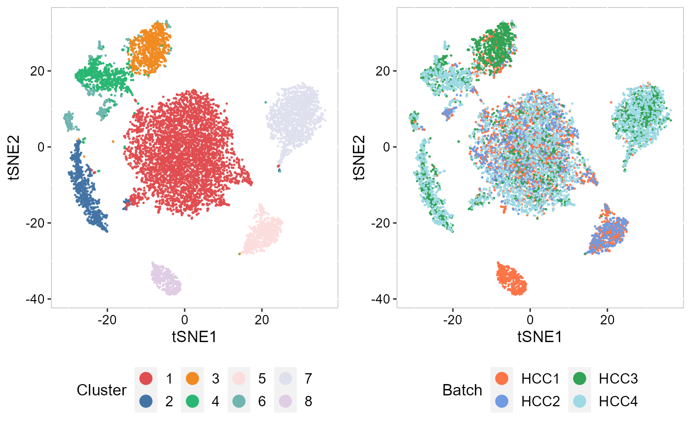
Spatial heatmap to show the clustering performance
Except for the embedding plots, SRTpipeline also provides a variaty of visualization functions. First, we visualize the spatial distribution of cluster labels that shows the layer structure for all data batches.
## choose colors to function chooseColors
p12 <- EachClusterSpaHeatMap(SRTProj, cols = cols_cluster, legend.position = "right", base_size = 12,
pt_size = 1, layout.dim = c(2, 2))
p12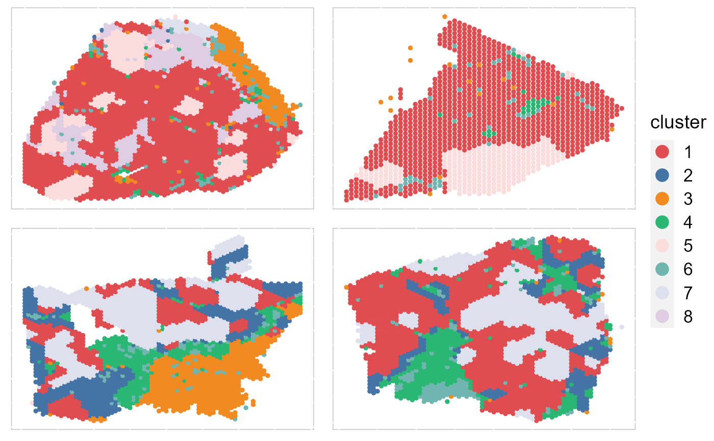 By setting
 combine =FALSE, this function will return a list of ggplot2 objects, thus user can revise each plot. In addtion, we can also plot some of data batches that are interested using the number ID or names of batch.
pList <- EachClusterSpaHeatMap(SRTProj, cols = cols_cluster, legend.position = "bottom", base_size = 12,
    pt_size = 0.5, layout.dim = c(2, 4), nrow.legend = 1, combine = FALSE)
EachClusterSpaHeatMap(SRTProj, batch = 1:3, title_name = "PRECAST: ", cols = cols_cluster, legend.position = "right",
    base_size = 12, pt_size = 1, layout.dim = c(2, 2))
EachClusterSpaHeatMap(SRTProj, batch = c("HCC1", "HCC2", "HCC3"), title_name = "PRECAST: ", cols = cols_cluster,
    legend.position = "right", base_size = 12, pt_size = 1, layout.dim = c(2, 2))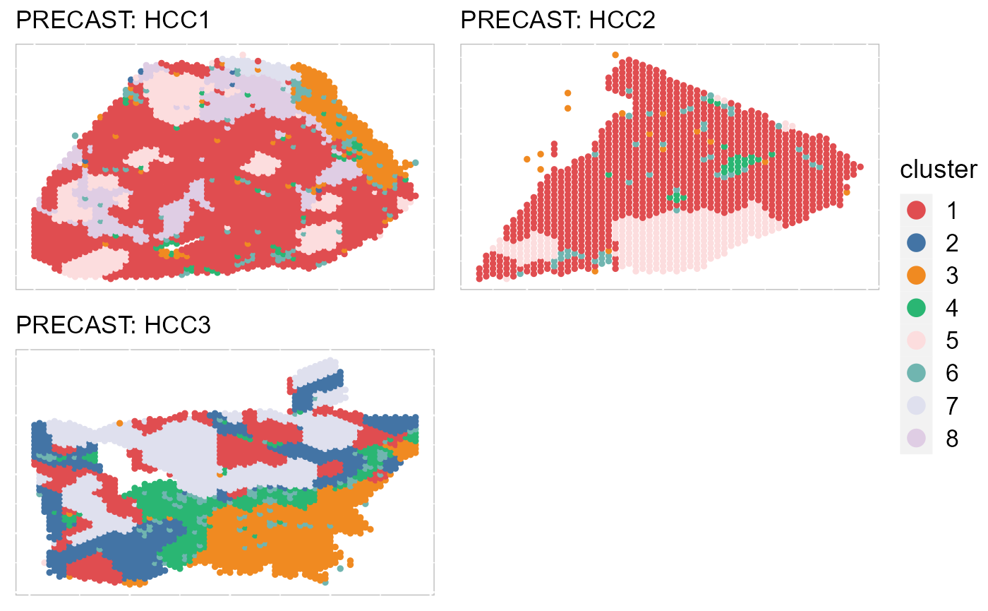
RGB plot to show the embedding performance
Next, we summarized the inferred embeddings for biological effects between spatial domain types (the slot reductions) using three components from either tSNE or UMAP and visualized the resulting tSNE/UMAP components with red/green/blue (RGB) colors in the RGB plot.
The resulting RGB plots from PRECAST showed the laminar organization of the human cerebral cortex, and PRECAST provided smooth transitions across neighboring spots and spatial domains.
SRTProj <- AddTSNE(SRTProj, n_comp = 3, reduction = "aligned.PRECAST")
p_tsne3 <- EachRGBSpaHeatMap(SRTProj, plot_type = "tSNE", pt_size = 0.5, title_name = "", layout.dim = c(2,
4))
p_tsne3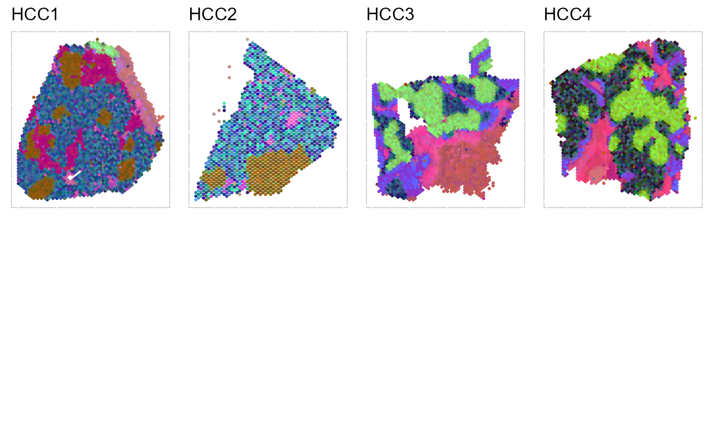 To run UMAP in SRTpipeline we use the
 AddUMAP() function. Frist, we evaluate the two-dimensional UMAPs.
SRTProj <- AddUMAP(SRTProj, n_comp = 2, reduction = "aligned.PRECAST")
p_umap2_cluster <- EmbedPlot(SRTProj, item = "cluster", plotEmbeddings = "UMAP", cols = cols_cluster,
legend.position = "bottom")
p_umap2_batch <- EmbedPlot(SRTProj, item = "batch", plotEmbeddings = "UMAP", cols = cols_batch,
legend.position = "bottom", nrow.legend = 2)
drawFigs(list(p_umap2_cluster, p_umap2_batch), layout.dim = c(1, 2), legend.position = "bottom")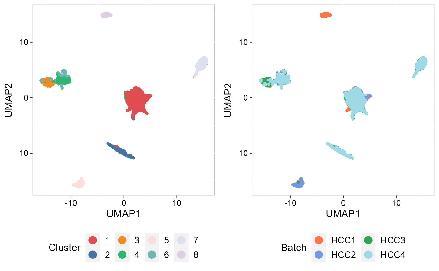 Then, we evaluate the three-dimensional UMAPs.
SRTProj <- AddUMAP(SRTProj, n_comp = 3, reduction = "aligned.PRECAST")
p_umap3 <- EachRGBSpaHeatMap(SRTProj, plot_type = "UMAP", layout.dim = c(2, 4), pt_size = 0.5, title_name = "UMAP: ")
p_umap3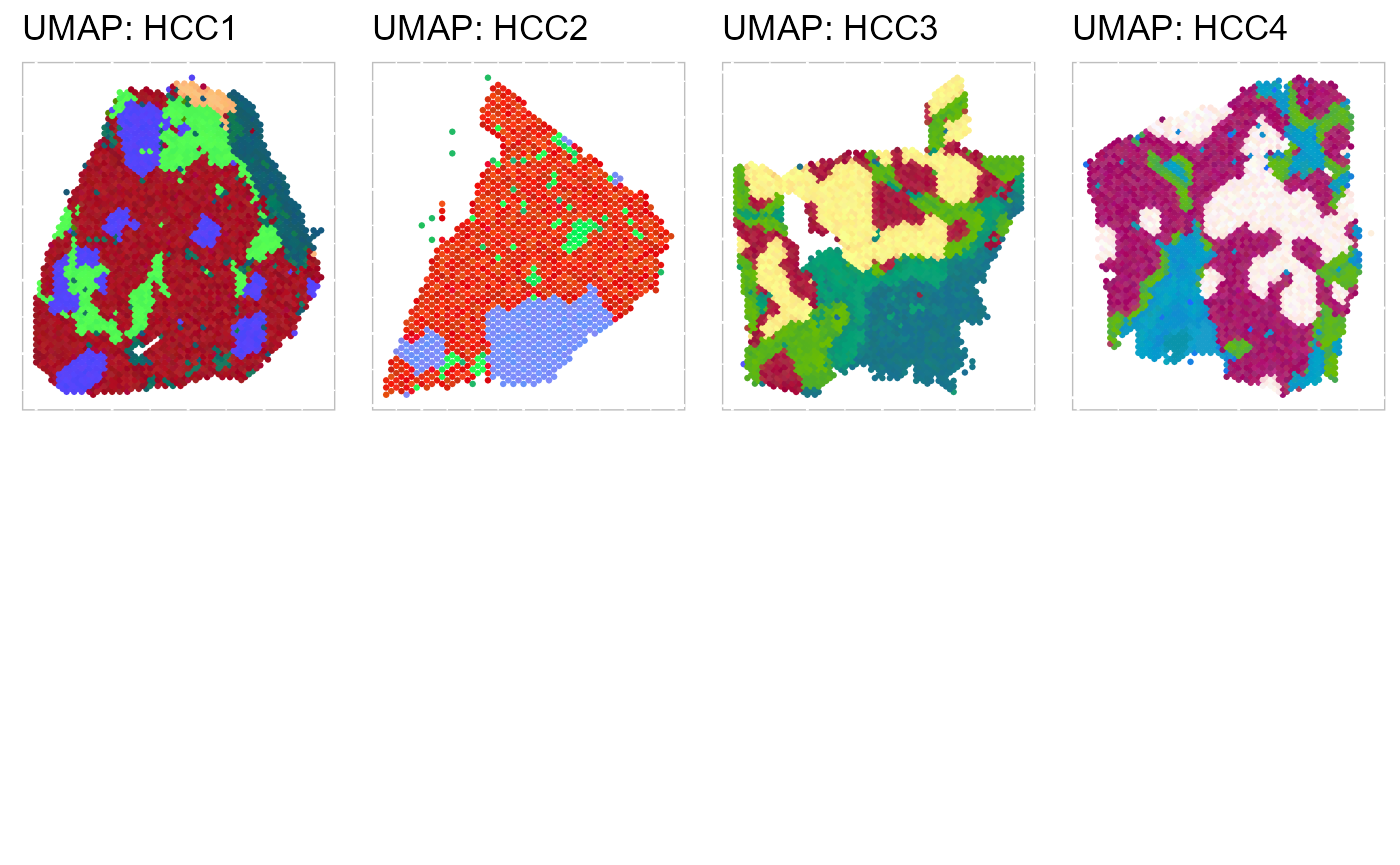
To save the plot, we can use write_fig() function.
write_fig(p_umap3, filename = "PRECAST_p_umap3.png", width = 14, height = 11)Moreover, we can visualize the microenvironment effects on the spatial coordinates. Then, we evaluate the three-dimensional UMAPs based on microEnv.PRECAST.
# save the previous calculated UMAP3
umap3_cluster <- SRTProj@plotEmbeddings$UMAP3
SRTProj <- AddUMAP(SRTProj, n_comp = 3, reduction = "microEnv.PRECAST")
p_umap3_micro <- EachRGBSpaHeatMap(SRTProj, plot_type = "UMAP", layout.dim = c(2, 4), pt_size = 1.2,
    title_name = "mircoEnv: ")
p_umap3_micro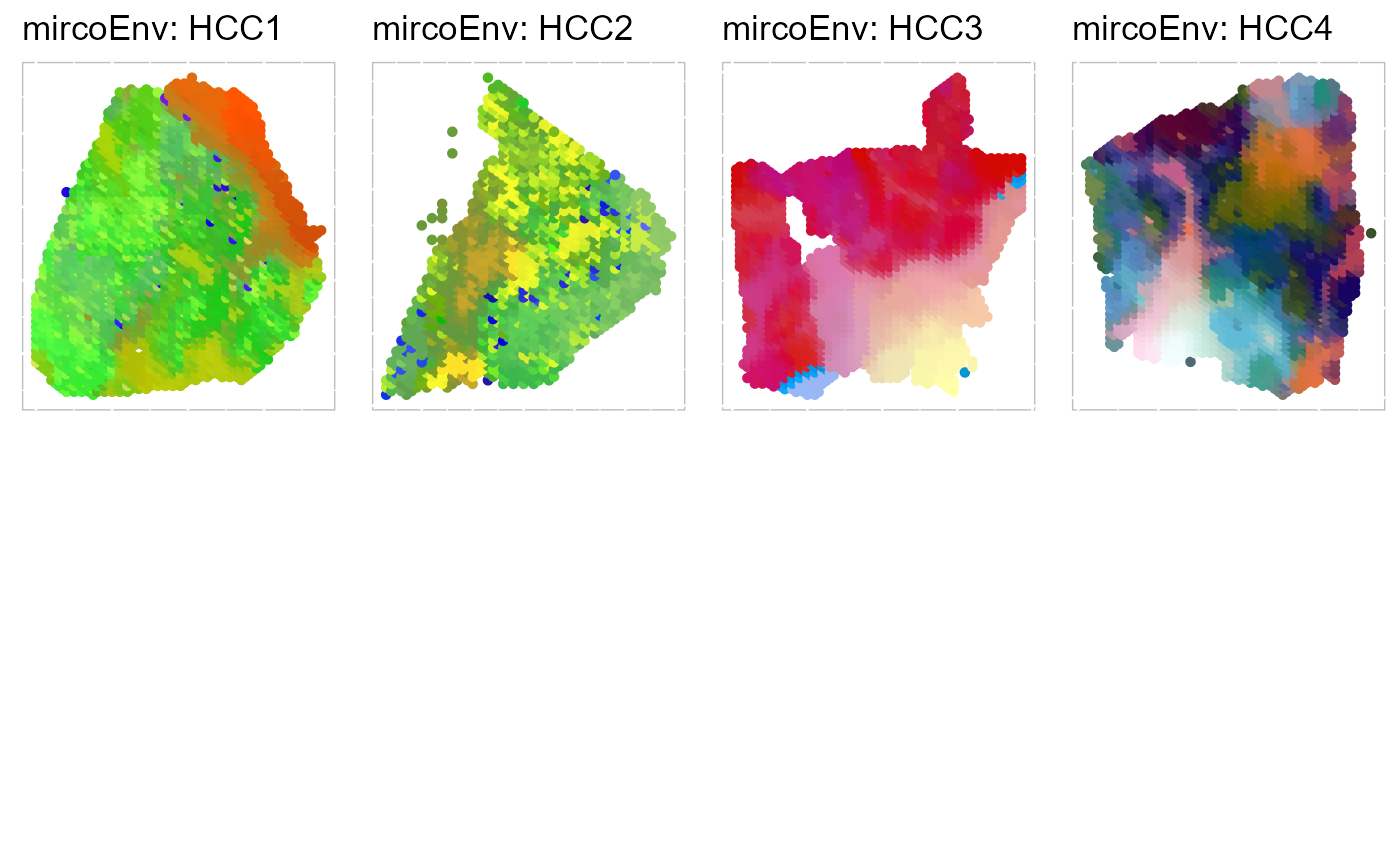
Cell-by-cell heatmap to show the relation of spatial domains
We plotted the heatmap of Pearson’s correlation coefcients of the estimated embeddings among the detected domains shows the good separation of the estimated embeddings across domains and the correlations between deeper layers were high, e.g., there were high correlations between domain 2 and 3, while correlations among the separated layers were low, i.e., domain 1 and 4.
p_cc <- CCHeatMap(SRTProj, reduction = "aligned.PRECAST", grp_color = cols_cluster)
p_cc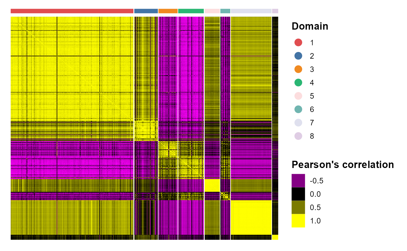 After adding the quantities for data visualization, the
 SRTProject object will have more information in the downstream analyses information. Now, we print this SRTProject object to check it. We observed two components added in the slot plotEmbeddings (Embeddings for plotting): tSNE, tSNE3, UMAP and UMAP3.
SRTProj## class: SRTProject
## outputPath: F:\Research paper\IntegrateDRcluster\AnalysisCode\SRTpipeline\vignettes\HCC4_PRECAST
## h5filePath: F:\Research paper\IntegrateDRcluster\AnalysisCode\SRTpipeline\vignettes\HCC4_PRECAST/HCC4_PRECAST.h5
## ---------Datasets basic information-----------------
## samples(4): HCC1 HCC2 HCC3 HCC4
## sampleColData names(3): species tissues NumOfSpots
## cellMetaData names(10): orig.ident nCount_RNA ... imagecol batch
## numberOfSpots(4): 2983 1334 2732 2764
## ---------Downstream analyses information-----------------
## Variable features: 2000
## Low-dimensional embeddings(2): microEnv.PRECAST aligned.PRECAST
## Inferred cluster labels: Yes
## Embedding for plotting(4): tSNE tSNE3 UMAP UMAP3Combined DEG analysis
After obtain the spatial cluster labels using a clustering model, we can perform differentially expression analysis. The argument only.var.features implies whether do batch correction for only variable features (default as TRUE).
speInt <- getIntegratedData(SRTProj, Method = "PRECAST", species = "Human", only.var.features = TRUE)We perform differential expression analysis for all clusters by using FindAllMarkers() function, then the DE genes’ information is saved in a data.frame object dat_degs.
dat_degs <- FindAllDEGs(speInt)
dat_degs
## DataFrame with 1289 rows and 7 columns
## p_val avg_log2FC pct.1 pct.2 p_val_adj cluster
## <numeric> <numeric> <numeric> <numeric> <numeric> <factor>
## CRP 0.00000e+00 0.260223 1.000 0.995 0.00000e+00 1
## LCN2 1.32523e-302 0.681233 0.842 0.658 2.65047e-299 1
## GPX2 7.25522e-277 0.300463 0.997 0.974 1.45104e-273 1
## THBS1 4.05417e-242 -0.337956 0.942 0.956 8.10833e-239 1
## SPINK1 9.47703e-239 0.612831 0.870 0.735 1.89541e-235 1
## ... ... ... ... ... ... ...
## CYP2A6.4 9.88942e-25 -0.333501 0.855 0.871 1.97788e-21 8
## ADAMTS1.4 1.12284e-23 -0.294081 0.693 0.835 2.24567e-20 8
## PTGDS.4 7.50928e-20 0.336822 1.000 0.933 1.50186e-16 8
## CCL2.5 4.99032e-16 -0.305413 0.751 0.816 9.98065e-13 8
## PPP1R3G 6.27300e-07 0.252607 0.603 0.617 1.25460e-03 8
## gene
## <character>
## CRP CRP
## LCN2 LCN2
## GPX2 GPX2
## THBS1 THBS1
## SPINK1 SPINK1
## ... ...
## CYP2A6.4 CYP2A6
## ADAMTS1.4 ADAMTS1
## PTGDS.4 PTGDS
## CCL2.5 CCL2
## PPP1R3G PPP1R3GWe identify the significant DE genes by two criteria: (a) adjustd p-value less than 0.01 and (b) average log fold change greater than 0.4.
degs_sig <- subset(dat_degs, p_val_adj < 0.01 & avg_log2FC > 0.5)
degs_sig
## DataFrame with 115 rows and 7 columns
## p_val avg_log2FC pct.1 pct.2 p_val_adj cluster
## <numeric> <numeric> <numeric> <numeric> <numeric> <factor>
## LCN2 1.32523e-302 0.681233 0.842 0.658 2.65047e-299 1
## SPINK1 9.47703e-239 0.612831 0.870 0.735 1.89541e-235 1
## CYP2A6.1 7.70864e-270 0.609182 0.999 0.858 1.54173e-266 2
## HAMP 1.04490e-209 0.589038 0.997 0.859 2.08981e-206 2
## APOF 4.64130e-192 0.537714 0.971 0.762 9.28259e-189 2
## ... ... ... ... ... ... ...
## CFHR5.1 1.13095e-156 0.579096 0.979 0.879 2.26189e-153 8
## GRAMD4.2 1.13217e-152 0.547481 0.998 0.919 2.26434e-149 8
## SPINK1.6 9.16304e-107 0.794890 1.000 0.787 1.83261e-103 8
## NQO1.5 3.72937e-81 0.506632 0.998 0.696 7.45874e-78 8
## CYP3A7.7 3.04553e-63 0.568287 1.000 0.817 6.09105e-60 8
## gene
## <character>
## LCN2 LCN2
## SPINK1 SPINK1
## CYP2A6.1 CYP2A6
## HAMP HAMP
## APOF APOF
## ... ...
## CFHR5.1 CFHR5
## GRAMD4.2 GRAMD4
## SPINK1.6 SPINK1
## NQO1.5 NQO1
## CYP3A7.7 CYP3A7In the following, we perform gene set enrichment analysis for the DE genes of each Domain identified by DR-SC model using R package gprofiler2.
library(gprofiler2)
termList <- list()
for (k in 1:8) {
    # k <- 1
    if (sum(degs_sig$cluster == k) > 0) {
        cat("k = ", k, "\n")
        dat_degs_sub <- subset(degs_sig, cluster == k)

        que1 <- dat_degs_sub$gene
        gostres <- gost(query = que1, organism = "hsapiens", correction_method = "fdr")
        termList[[k]] <- gostres
    }

}
## k = 1
## k = 2
## k = 3
## k = 4
## k = 5
## k = 6
## k = 7
## k = 8
head(termList[[1]]$result)## query significant p_value term_size query_size intersection_size
## 1 query_1 TRUE 0.02257092 7 2 1
## 2 query_1 TRUE 0.02257092 10 2 1
## 3 query_1 TRUE 0.02257092 6 2 1
## 4 query_1 TRUE 0.02257092 9 2 1
## 5 query_1 TRUE 0.02257092 7 2 1
## 6 query_1 TRUE 0.02257092 14 2 1
## precision recall term_id source
## 1 0.5 0.14285714 GO:0090186 GO:BP
## 2 0.5 0.10000000 GO:0090281 GO:BP
## 3 0.5 0.16666667 GO:0097577 GO:BP
## 4 0.5 0.11111111 GO:1900003 GO:BP
## 5 0.5 0.14285714 GO:1902572 GO:BP
## 6 0.5 0.07142857 GO:1901678 GO:BP
## term_name effective_domain_size
## 1 regulation of pancreatic juice secretion 21092
## 2 negative regulation of calcium ion import 21092
## 3 sequestering of iron ion 21092
## 4 regulation of serine-type endopeptidase activity 21092
## 5 negative regulation of serine-type peptidase activity 21092
## 6 iron coordination entity transport 21092
## source_order parents
## 1 21177 GO:0030157, GO:0044058, GO:0050878, GO:0051046
## 2 21267 GO:0051926, GO:0070509, GO:0090279
## 3 21858 GO:0006879, GO:0051238, GO:0051651
## 4 23354 GO:0052548, GO:1902571
## 5 25729 GO:0010466, GO:1902571
## 6 24939 GO:0006826To understand the functions of the identified spatial domains by DR-SC model, we compare the top significant biological process (BP) pathways in GO database for the DE genes from Domain 1 and 2. Here, we only show to visualize the significant BP pathways and users can explore the other databases such as KEGG and HPA.
## Most commonly used databases
source_set <- c("GO:BP", "GO:CC", "GO:MF", "KEGG", "HPA")
cols <- c("steelblue3", "goldenrod", "brown3", "#f98866", "#CE6DBD")
## Here, we show GO:BP
source1 <- "GO:BP"
ss <- which(source_set == source1)
ntop = 5
names(cols) <- source_set
pList_enrich <- list()
for (ii in 1:5) {
    ## ii <- 5
    message("ii=", ii)
    gostres2 <- termList[[ii]]
    if (!is.null(gostres2$result)) {
        dat1 <- subset(gostres2$result, term_size < 500)
        dat1 <- get_top_pathway(dat1, ntop = ntop, source_set = source1)
        dat1 <- dat1[complete.cases(dat1), ]
        dat1$nlog10P <- -log10(dat1$p_value)

        pList_enrich[[ii]] <- barPlot_enrich(dat1[order(dat1$nlog10P), ], source = "source", "term_name",
            "nlog10P", cols = cols[source_set[ss]], base_size = 14) + ylab("-log10(p-adj)") + xlab("Biological terms") +
            ggtitle(paste0("Domain", ii))
    }
}
drawFigs(pList_enrich[c(1, 4)], layout.dim = c(2, 1), common.legend = T, align = "hv")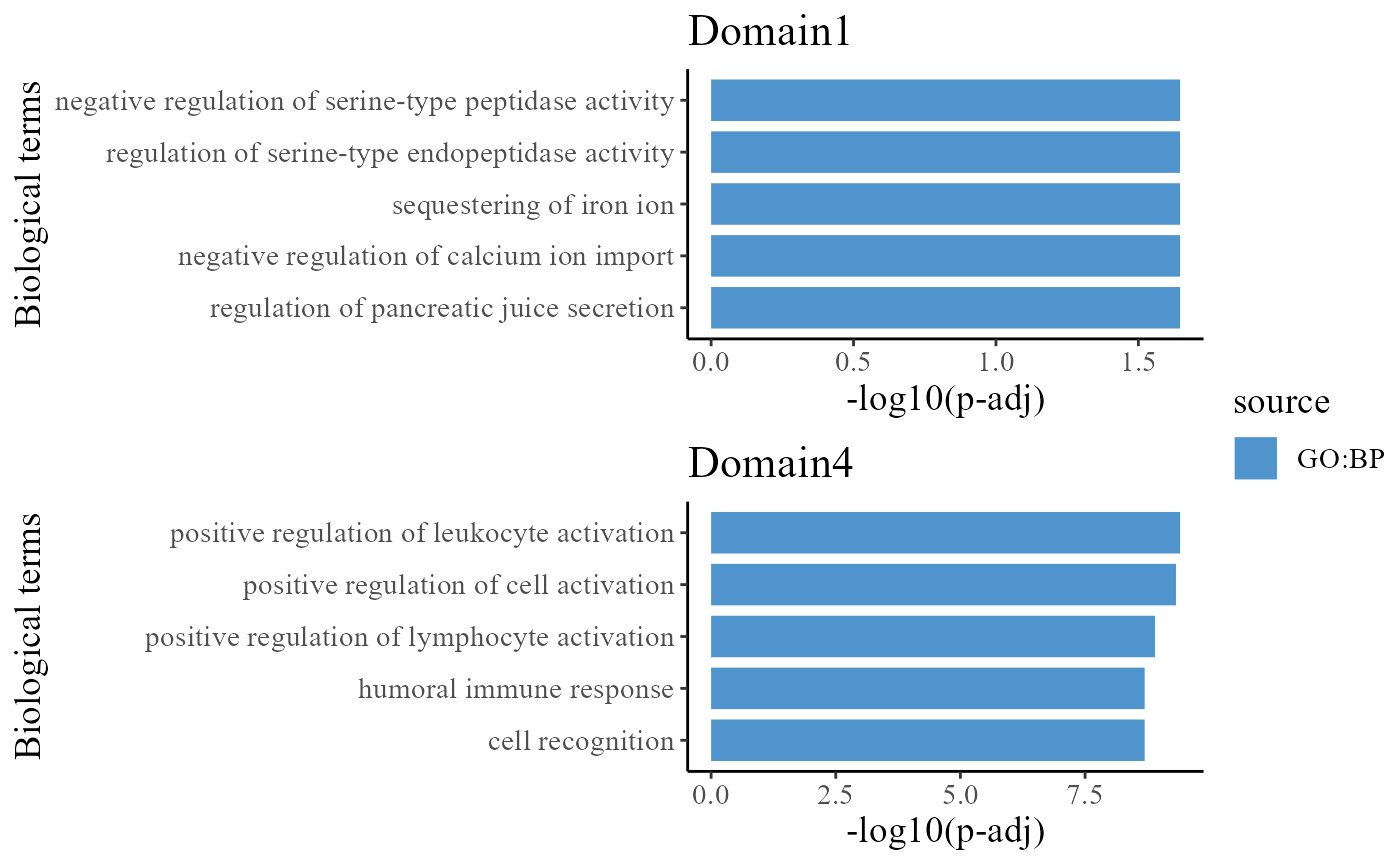
We take out the top DE genes for each cluster for visualization.
library(dplyr)
n <- 5
dat_degs %>%
    as.data.frame %>%
    group_by(cluster) %>%
    top_n(n = n, wt = avg_log2FC) -> topGene
topGene
## # A tibble: 40 x 7
## # Groups: cluster [8]
## p_val avg_log2FC pct.1 pct.2 p_val_adj cluster gene
## <dbl> <dbl> <dbl> <dbl> <dbl> <fct> <chr>
## 1 1.33e-302 0.681 0.842 0.658 2.65e-299 1 LCN2
## 2 9.48e-239 0.613 0.87 0.735 1.90e-235 1 SPINK1
## 3 2.98e-220 0.492 0.896 0.766 5.96e-217 1 CYP3A7
## 4 1.38e-209 0.482 0.816 0.629 2.75e-206 1 GPC3
## 5 1.11e-177 0.487 0.85 0.715 2.21e-174 1 AKR1B10
## 6 7.71e-270 0.609 0.999 0.858 1.54e-266 2 CYP2A6
## 7 1.04e-209 0.589 0.997 0.859 2.09e-206 2 HAMP
## 8 4.64e-192 0.538 0.971 0.762 9.28e-189 2 APOF
## 9 2.49e-185 0.556 0.999 0.858 4.99e-182 2 MT1E
## 10 4.42e-137 0.604 0.999 0.907 8.84e-134 2 RBP4
## # ... with 30 more rowsWe visualize the DE genes for each cluster group by gene-by-cell heatmap using the GCHeatMap() function.
p1 <- GCHeatMap(speInt, features = topGene$gene, grp_color = cols_cluster, y_text_size = 10)
p1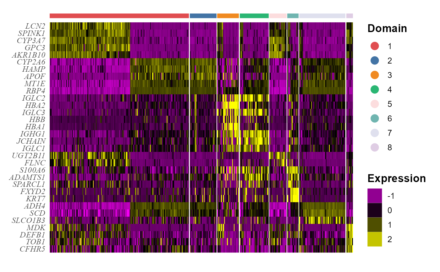
Trajectory inference
Next, we performed trajectory inference using the aligned embeddings and domain labels estimated by PRECAST model.
speInt <- AddTrajectory(speInt, reduction = "aligned.PRECAST")
p1 <- EmbedPlot(speInt, plotEmbeddings = "aligned.PRECAST", colour_by = "PT")
p2 <- EmbedPlot(speInt, plotEmbeddings = "tSNE", colour_by = "PT")
drawFigs(list(p1, p2), layout.dim = c(1, 2), common.legend = TRUE, legend.position = "right")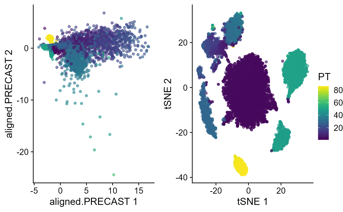
Visualize the inferred pseudotime on the spatial coordinates for each data batch.
p_spa <- EachEmbedPlot(speInt, reduction = "Coord", colour_by = "PT", layout.dim = c(2, 4))
p_spa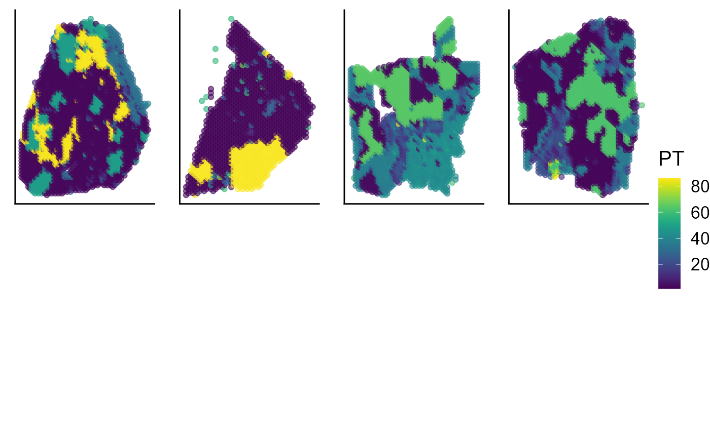
# save(SRTProj, file=paste0(SRTProj@projectMetadata$outputPath,'/SRTProj.rds'))
# load('F:/Research
# paper/IntegrateDRcluster/AnalysisCode/SRTpipeline/vignettes/Liver8/SRTProj.rds')
Other downstream analyses
Session Info
## R version 4.1.2 (2021-11-01)
## Platform: x86_64-w64-mingw32/x64 (64-bit)
## Running under: Windows 10 x64 (build 22621)
##
## Matrix products: default
##
## locale:
## [1] LC_COLLATE=Chinese (Simplified)_China.936
## [2] LC_CTYPE=Chinese (Simplified)_China.936
## [3] LC_MONETARY=Chinese (Simplified)_China.936
## [4] LC_NUMERIC=C
## [5] LC_TIME=Chinese (Simplified)_China.936
##
## attached base packages:
## [1] stats4    stats     graphics  grDevices utils     datasets  methods
## [8] base
##
## other attached packages:
##  [1] scater_1.25.1               scuttle_1.4.0
##  [3] slingshot_2.2.0             TrajectoryUtils_1.2.0
##  [5] princurve_2.1.6             gprofiler2_0.2.1
##  [7] bigalgebra_1.1.0            bigmemory_4.5.36
##  [9] SpatialExperiment_1.4.0     SingleCellExperiment_1.16.0
## [11] SummarizedExperiment_1.24.0 Biobase_2.54.0
## [13] GenomicRanges_1.46.1        GenomeInfoDb_1.30.1
## [15] IRanges_2.28.0              MatrixGenerics_1.6.0
## [17] matrixStats_0.62.0          dplyr_1.0.9
## [19] ggplot2_3.3.6               colorspace_2.0-3
## [21] Matrix_1.4-0                hdf5r_1.3.5
## [23] ff_4.0.7                    bit_4.0.4
## [25] S4Vectors_0.32.3            BiocGenerics_0.40.0
## [27] rhdf5_2.38.0                sp_1.5-0
## [29] SeuratObject_4.1.0          Seurat_4.1.1
## [31] SRTpipeline_0.1.1
##
## loaded via a namespace (and not attached):
##   [1] scattermore_0.8           ggthemes_4.2.4
##   [3] R.methodsS3_1.8.1         GiRaF_1.0.1
##   [5] ragg_1.2.2                tidyr_1.2.0
##   [7] bit64_4.0.5               knitr_1.37
##   [9] irlba_2.3.5               DelayedArray_0.20.0
##  [11] R.utils_2.11.0            data.table_1.14.2
##  [13] rpart_4.1.16              RCurl_1.98-1.6
##  [15] generics_0.1.2            ScaledMatrix_1.2.0
##  [17] cowplot_1.1.1             RANN_2.6.1
##  [19] future_1.26.1             spatstat.data_3.0-0
##  [21] httpuv_1.6.5              assertthat_0.2.1
##  [23] viridis_0.6.2             xfun_0.29
##  [25] jquerylib_0.1.4           evaluate_0.15
##  [27] promises_1.2.0.1          fansi_1.0.3
##  [29] igraph_1.3.5              DBI_1.1.2
##  [31] htmlwidgets_1.5.4         spatstat.geom_2.4-0
##  [33] purrr_0.3.4               ellipsis_0.3.2
##  [35] RSpectra_0.16-1           ggpubr_0.4.0
##  [37] backports_1.4.1           DR.SC_3.1
##  [39] deldir_1.0-6              sparseMatrixStats_1.6.0
##  [41] vctrs_0.4.1               ROCR_1.0-11
##  [43] abind_1.4-5               cachem_1.0.6
##  [45] withr_2.5.0               PRECAST_1.4
##  [47] progressr_0.10.1          sctransform_0.3.3
##  [49] mclust_5.4.10             goftest_1.2-3
##  [51] cluster_2.1.2             lazyeval_0.2.2
##  [53] crayon_1.5.1              SpatialAnno_1.0.0
##  [55] edgeR_3.36.0              pkgconfig_2.0.3
##  [57] labeling_0.4.2            nlme_3.1-155
##  [59] vipor_0.4.5               rlang_1.0.2
##  [61] globals_0.15.0            lifecycle_1.0.1
##  [63] miniUI_0.1.1.1            bigmemory.sri_0.1.3
##  [65] rsvd_1.0.5                rprojroot_2.0.3
##  [67] polyclip_1.10-0           lmtest_0.9-40
##  [69] SC.MEB_1.1                carData_3.0-5
##  [71] Rhdf5lib_1.16.0           zoo_1.8-10
##  [73] beeswarm_0.4.0            ggridges_0.5.3
##  [75] rjson_0.2.21              png_0.1-7
##  [77] viridisLite_0.4.0         iSC.MEB_1.0.1
##  [79] bitops_1.0-7              R.oo_1.24.0
##  [81] KernSmooth_2.23-20        rhdf5filters_1.6.0
##  [83] DelayedMatrixStats_1.16.0 stringr_1.4.0
##  [85] parallelly_1.32.0         spatstat.random_2.2-0
##  [87] rstatix_0.7.0             ggsignif_0.6.3
##  [89] beachmat_2.10.0           scales_1.2.0
##  [91] memoise_2.0.1             magrittr_2.0.3
##  [93] plyr_1.8.7                ica_1.0-2
##  [95] zlibbioc_1.40.0           compiler_4.1.2
##  [97] dqrng_0.3.0               RColorBrewer_1.1-3
##  [99] fitdistrplus_1.1-8        cli_3.2.0
## [101] XVector_0.34.0            listenv_0.8.0
## [103] patchwork_1.1.1           pbapply_1.5-0
## [105] formatR_1.11              MASS_7.3-55
## [107] mgcv_1.8-39               tidyselect_1.1.2
## [109] stringi_1.7.6             textshaping_0.3.6
## [111] highr_0.9                 yaml_2.3.6
## [113] locfit_1.5-9.4            BiocSingular_1.10.0
## [115] ggrepel_0.9.1             grid_4.1.2
## [117] sass_0.4.1                tools_4.1.2
## [119] future.apply_1.9.0        parallel_4.1.2
## [121] rstudioapi_0.13           gridExtra_2.3
## [123] farver_2.1.0              Rtsne_0.16
## [125] DropletUtils_1.14.2       digest_0.6.29
## [127] rgeos_0.5-9               shiny_1.7.1
## [129] Rcpp_1.0.10               car_3.0-12
## [131] broom_0.7.12              later_1.3.0
## [133] RcppAnnoy_0.0.19          httr_1.4.3
## [135] fs_1.5.2                  tensor_1.5
## [137] reticulate_1.25           splines_4.1.2
## [139] uwot_0.1.11               spatstat.utils_3.0-1
## [141] pkgdown_2.0.6             plotly_4.10.0
## [143] systemfonts_1.0.4         xtable_1.8-4
## [145] jsonlite_1.8.0            R6_2.5.1
## [147] pillar_1.7.0              htmltools_0.5.2
## [149] mime_0.12                 glue_1.6.2
## [151] fastmap_1.1.0             BiocParallel_1.28.3
## [153] BiocNeighbors_1.12.0      codetools_0.2-18
## [155] utf8_1.2.2                lattice_0.20-45
## [157] bslib_0.3.1               spatstat.sparse_2.1-1
## [159] tibble_3.1.7              ggbeeswarm_0.6.0
## [161] leiden_0.4.2              gtools_3.9.2.2
## [163] magick_2.7.3              limma_3.50.1
## [165] survival_3.2-13           CompQuadForm_1.4.3
## [167] rmarkdown_2.11            desc_1.4.0
## [169] munsell_0.5.0             GenomeInfoDbData_1.2.7
## [171] HDF5Array_1.22.1          reshape2_1.4.4
## [173] gtable_0.3.0              spatstat.core_2.4-4